Professor
Mike Veatch
MAT220B
Biostatistics: Kinesiology project
Introduction
The
purpose of this study is to evaluate the validity of a study involving men,
women, weight, and metabolic rate. I will calculate regression of the
relationships between these variables. I will also ask what type of
relationship these variables have, linear, quadratic? Also, what is the best
type of equation to model these variables with, one with multiple or a single
variable?
Data Collection
Metabolic
rate is a measurement that reports kilocalories burned per 24 hours.
[1]
This can be measured with a few different methods; the most accurate is
indirect calorimetry. Easier, but less
accurate is the use of a device such as the BodyGem,
and the easiest of all is to use an equation, such as the Weir equation.
[2]
Answers
1.
The
results may be affected by the fact that the subjects were dieting. Certain
subjects may shift in metabolic rate as a reaction to the changed diet more
than other subjects. This could create lower correlation in data by having a
spread of subjects, some of which fluctuate more than others in metabolic rate
as a reaction the changed diet.
2.
The
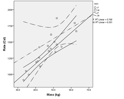
regression lines for the males has a lower slope than
the female regression line, meaning that the male rate is greater than the
female rate at low body mass (Fig. 1). The male average rate is greater than
the female average rate. The greater y-intercept could be because males have a
greater baseline metabolic rate, while the greater slope associated with the
female regression line slope could be attributed to their small body mass that
as it increases, the rate needs to greatly adjust to compensate for their
smaller initial metabolic rate. The correlation for females is much stronger
than for males (.768 female vs. .351 male). This could be because there is
greater variation in male metabolic rate, which assumes good data collection.
Figure
1. Scatterplot of mass (explanatory) vs. metabolic rate (response). 95%
confidence intervals included.
3.
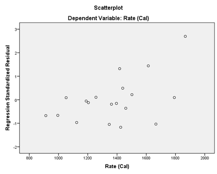
The
three conditions for inference are normal residuals, linearity, and constant
standard deviation.
[3]
There is a violation of constant standard deviation, because the spread of
points starts small, but becomes larger as y values increase. Linearity is not
violated, however, there may be slight concave down curve for the male
relationship between mass and metabolic rate. More points exist below the line
of regression than above, and if I imagine a line slightly curved concave down
a better fit may be found for this data. Based on the same logic, there does
not seem to be a curve in the line for the female relationship, because the
spread of points seems evenly distributed above and below the line of
regression. There is not a violation of normal residuals, because if a y = 0
line is drawn, a line with no slope that originates at y = 0, about half of the
points fall on either side of this line, making it a normal distribution. The
point at the top right of the graph may be an outlier, but if the regression
line of this chart has a positive slope, it may not be too far from the
regression line; its residual may not be much greater than the average residual
length.
Figure
2. Rate (explanatory variable) vs. regression standardized residual for a
regression between rate and mass.
4.
H0
= there is no correlation between mass and rate. Ha = there is a
correlation between mass and rate. Rate and sex do have a relationship, and so
do rate and mass, because both of them have significance values below the alpha
level of 0.1.
[4]
The equation of this multiple regression is
. For the indicator variable,
female = 1, and male = 0. Using this formula, we can calculate the mean rate
for a 45kg female:
, yields y = 1276.55. The p value
is below 0.05 ( p < 0.000 ), therefore we conclude
that there is significant correlation between these variables.
5.
The
R2 from a regression involving mass and sex as explanatory variables
and rate as a response variable is 0.799. The R2 between mass and
rate yields an R2 of 0.748. The R2 between sex and rate
is 0.493. The R2 between interaction and rate is 0.312. Therefore,
the model including mass and sex as explanatory variables gives the greatest
correlation. All three of these tests have significance levels below 0.1, so a
linear relationship models all of these variables well.
However, the R2 of the interaction as explanatory variable is too
low (0.312) to make for a decent model.
6.
In
figure 1, I present a scatterplot of weight (explanatory) vs. rate (response)
in which there is graphed onto the plot a confidence interval (CI) of 95%.
These confidence intervals tell us that we can predict with 95% confidence that
the mean rate is between the CI lines. The CI for females is more accurate—more
narrow than the CI for males.
Conclusions
I
found significant relationships between all of the
variables, as evidenced by the P values yielded by the regression tests I
performed. The regression with mass and sex as explanatory variables has a p
value less than 0.000, with interaction as an explanatory variable gives a p
value of 0.013, of mass only yields less than 0.000, and of sex equals 0.001.
Works
Cited
Brigitte
Baldi, D. S. (2012). The Practice of Statistics in the LIfe SCiences.
New York, NY: W.H. Freeman and Company.
Kelly,
M. P. (2014). Resting Metabolic Rate: Best Ways to Measure It—And Raise It,
Too. Retrieved April 25, 2014, from American Council on Exercise:
http://www.acefitness.org/certifiednewsarticle/2882/resting-metabolic-rate-best-ways-to-measure-it-and/


